For complete understanding of a problem and to improve in the future, thorough analysis is needed both before implementing a solution and in understanding how one performs. While the Data page introduced the dataset and certain engineered features, select exploratory data analysis is instead included here as it also relates to understanding and performance. Importantly, from the beginning it could be seen that elevation would be one of the most important variables in the problem.

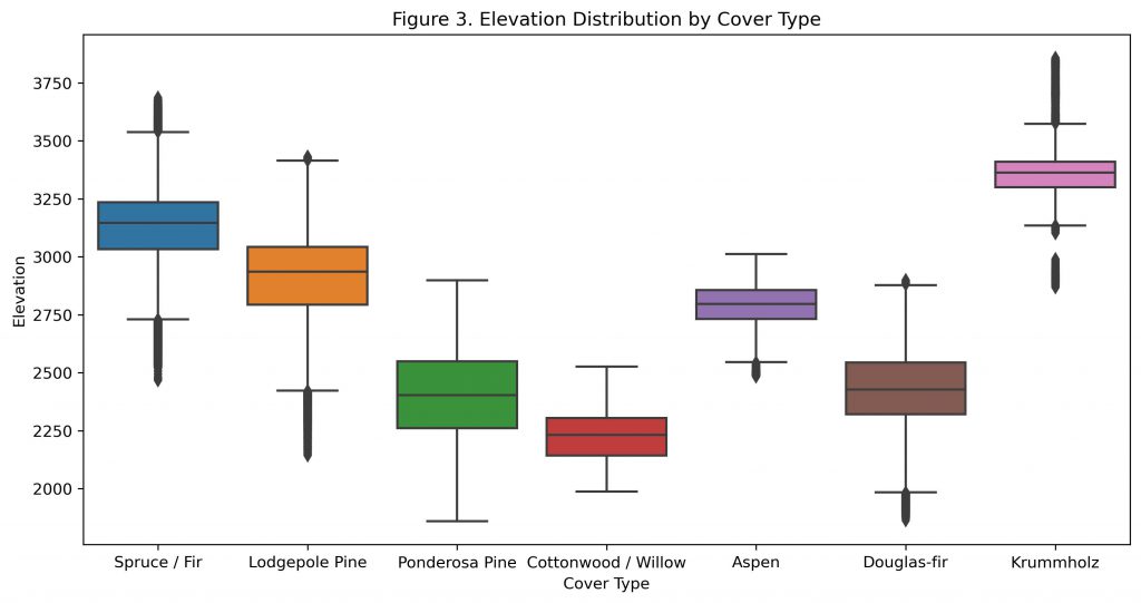
Figure 3 shows how almost every cover type has a median elevation that is unique and does not overlap with the middle 50% of observations from any other cover type. The only exception to this are the Cottonwood / Willow and Douglas-fir cover types, which have nearly identical elevation distributions. This makes it a distinct feature and one that would be important to any potential solution.

To compare this variable to the others available, a principal component analysis can be conducted. Note that although principal component analysis relies on all variables being continuous, the independent categorical variables (i.e. wilderness area and soil type) can be encoded as a series of binary indicator variables as an approximation. For a similar but more correct treatment of a mix of continuous and categorical independent variables, multiple factor analysis may be conducted.

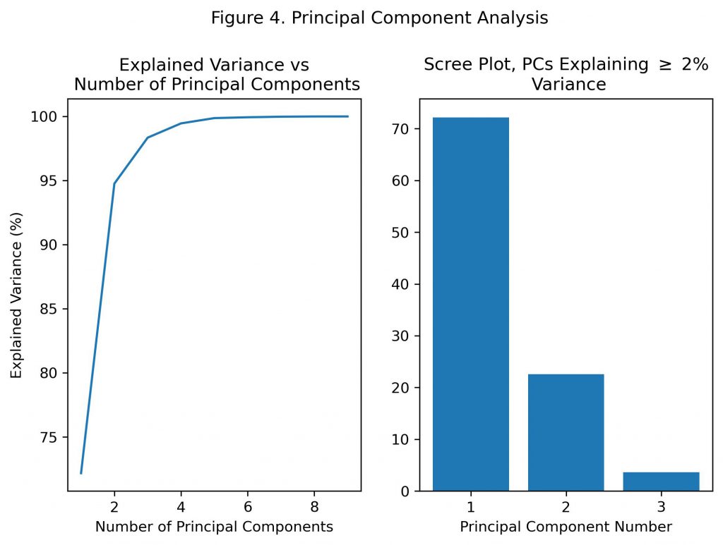
Figure 4 shows the results from a principal component analysis, which can be used to evaluate the general importance of elevation along with the other variables in the dataset. Principal component analysis takes successive linear combinations of the independent variables, where each combination explains the most remaining variance among the set of observations. It can be seen that with just one principal component, over 70% of the variance in the observations of the dataset is explained. The coefficients of the first principal component can be viewed as one way of judging feature importance.

Feature	Loading Score
Horizontal Distance to Roadways	0.81
Horizontal Distance to Fire Points	0.56
Elevation	0.18
Others	<0.05 each

Table 2 shows the loading scores of the first principal component. Only the three variables with the greatest magnitudes of loading scores are shown. For a given principal component, the loading score is the coefficient in the linear combination that is computed for each variable. Thus, higher loading scores indicate that the variable plays a greater role in explaining the remaining variance at the given principal component number. When examining the first principal component, the remaining variance is the entire variance of the dataset.

It can be seen that elevation had the third highest loading score, reinforcing its importance in differentiating the observations. The only two variables with higher loading scores are both related to human activity. Roadways are obviously human made, while fire points represent locations where a previous forest fire was started. Although there can be natural causes of forest fires, human activity is also a potential source and it is likely some fire points were from human causes. Since the dataset was intended to represent locations which are far from human activity, the few locations which are close to these features would be highly correlated and easily separable from the others based on these variables. If this is true, then elevation can be considered the most important naturally occurring variable in the dataset. This would also make it the most important for making future predictions, since the correlation between human-related variables and cover type may be spurious.

Indeed, by increasing the influence of elevation across models performance generally increased. For example, in the K-Nearest Neighbors model, this variable was multiplied by a constant factor after normalization so that differences in elevation would contribute to the Euclidean distance more so than other variables. To improve this project further or in new related applications, this variable should be throughly investigated.

To investigated and engineer features, other relationships between variables in the dataset were also investigated.

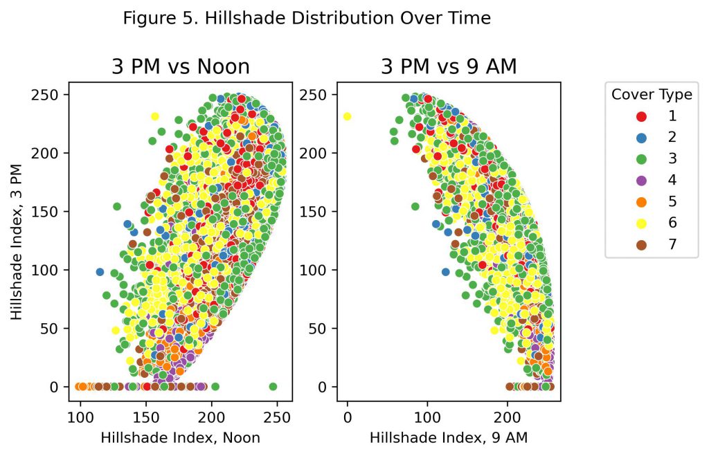
Figure 5 shows the distribution of the hillshade index at 3 PM compared to the two earlier times in the day. As mentioned on the Data page, although the variable is a “hillshade index”, higher values actually correspond to greater surface illumination while lower values correspond to greater shade. For each plot there is a clear curvature, with all cover types following the same trends. In the first, there is a positive correlation where the index at 3 PM generally increases as the index at noon increases. In the second, there is a negative correlation where the index at 3 PM generally decreases as the index at 9 AM increases. These opposite correlations are intuitive when aspect and slope are considered for how they would affect surface illumination. For example, a plot that faces the East will receive more sun in the morning and less in the afternoon. This would correspond to points towards the bottom of both plots, where afternoon illumination is lower. A plot facing the West, on the other hand, will experience more sun in the afternoon compared to the morning. These points would generally be located towards the top of both plots, where surface illumination at 3 PM is the greatest.

In each, it can also be seen that there are certain points which have a positive hillshade index at 9 AM or noon, but a hillshade index of zero at 3 PM. It is possible that these are either mistakes in annotation, or actually correspond to real points. In general settings, outliers clearly deviating from the main pattern are commonly incorrect or the result of filling in missing values by a previous author. On the other hand, it would be possible to imagine a scenario where early morning surface illumination could be non-zero but then shift to zero later in the day. For example, if a plot is located at the base of a cliff or sharp rise in elevation, then once the sun passes beyond the edge of its surroundings the plot would receive no direct sunlight. To better evaluate if this would be possible for these points, precise examples of hillshade index in other settings should be found. For example, if a zero hillshade index only requires no direct sunlight, it would be possible for these points to be real. If a zero hillshade index is only used for complete darkness, however, then this would likely not happen at any point during a normal day.

From domain knowledge, it was also expected that aspect may be related to the type of forest growth.

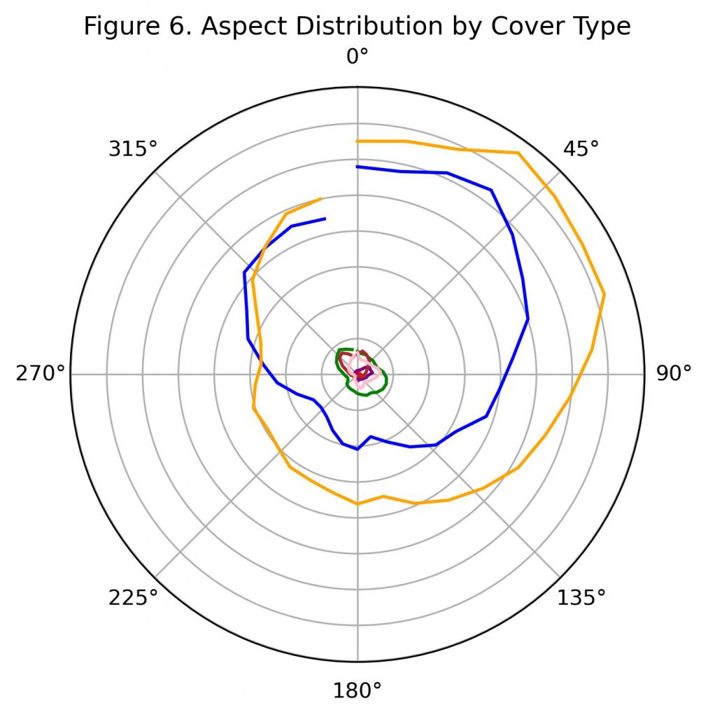
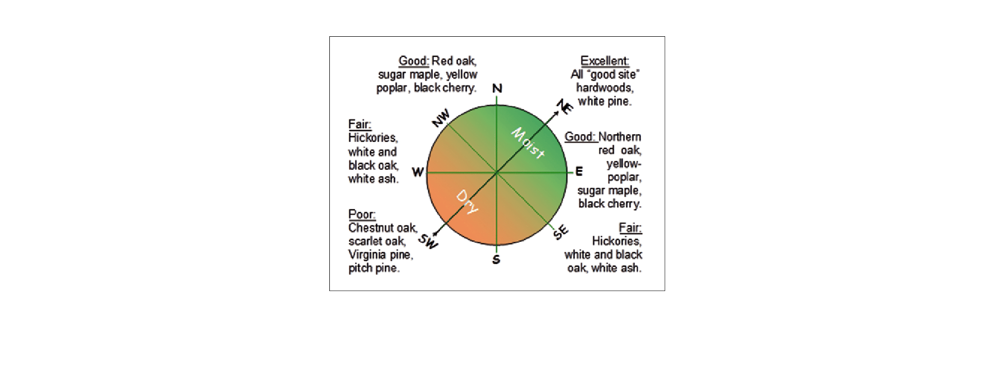
Figure 6 shows how the number of observations for each cover type, represented by the radial distance, varies with aspect. Figure 7 shows a similar diagram based on a study in Appalachian forests by the US Forest Service. As explained on the Data page, aspect indicates which direction a slope is facing, while degrees azimuth represents the clockwise degrees away from North. For example, an aspect of 180 degrees azimuth indicates a slope is facing due South.

The US Forest Service study focused on reforestation strategies in areas formerly used for mining, and suggests that aspect influences growth conditions. Specifically, the study found that areas with an aspect between 0 and 90 degrees azimuth is associated with the most “Excellent” tree growth potential by having greater soil moisture and sunlight. This in turn would affect the recommended trees that are planted for reforestation in these areas, as well as others where conditions are not as favorable.

These findings also reinforce the importance of aspect and its relationship to forest cover in this project. It can be seen in Figure 6 that the two most common forest covers, Spruce / Fir and Lodgepole Pine, are both more prevalent in the range with excellent growth potential. Although the species of trees are different across forests, the sole Spruce tree in the US Forest Service study, Red Spruce, was recommended for this range of azimuth as well. Others in this project, such as Cottonwood / Willow or Aspen, are less prevalent in the “Excellent” range and more often in the “Fair” or “Good” region. However, the study states that its own Aspen or Cottownwood species are also recommended for moist or wet conditions that are associated with better, rather than mediocre, growth. This demonstrates that with only qualitative comparisons, and the large magnitude of differences between forests or regions, there is a limit what knowledge can be transferred without expert knowledge or a deeper investigation.

Further work should be done to compare how the importance of aspect and growth conditions could vary across locations, such as from the Appalachians to Roosevelt National Forest in Colorado. It is likely that the relationship between aspect and growth is due to the longitude and latitude of the location on Earth and how that affects received sunlight. Therefore, the importance of aspect could change from one location in the country to another far away. The magnitude of recorded slopes in this dataset should also be compared to previous publications. For example, the same US Forest Service study broadly divides tree recommendations into whether an area is flat or sloped. With slope information recorded in this dataset, the slope or aspect-slope can specifically be compared to the recorded tables in US Forest Service study. Finally, the work done to aggregate the dataset originally could also be repeated for other forests recorded by the US Forest Service or Geological Survey. With multiple similar datasets across regions, better information could be extracted as to what trends in forest cover are general and what are specific to certain areas.

Citations:
[1] Franklin, Jennifer & Adams, Mary & Angel, Patrick & Barton, Christopher & Burger, J. & Davis, Vic & French, Michael & Graves, Don & Groninger, John & Hall, Nathan & Keiffer, Carolyn & Larkin, Jeffery & McCarthy, Brian & Miller, Christopher & Mizel, Jeremy & Skousen, Jeffrey & Strahm, Brian & Sweigard, Richard & Wood, Petra & Zipper, Carl. (2017). The Forestry Reclamation Approach: Guide to Successful Reforestation of Mined Lands. 10.2737/NRS-GTR-169.