With a fixed number of forest cover types, this is a classification problem. Classification is generally easier than more abstract tasks in machine learning, as there is a natural limit to the number of outputs a model can choose from. There are many potential metrics used in classification, but the original competition used accuracy for its leaderboard. An advantage of using accuracy is that it is easy to understand, and provides an overview of performance across all data. This is related to its disadvantages, however, being that specific trends or fine grained information on performance is lost at such a high level.

In classification scenarios, a natural baseline to judge performance against is to pick out the most common category and naively predict all data points as belonging to it. For example, if 90% of the data belonged to only one forest cover type, then assigning that type to all datapoints would result in an accuracy of 90%. This may sound impressive without knowledge of the imbalanced dataset, but does not represent any meaningful insight.

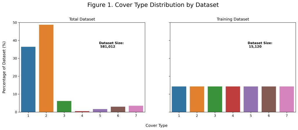
Figure 1 shows the distribution of forest cover types in the total and training datasets. In other circumstances, characteristics of the total or testing datasets may be unknown. In this project, because any use case would be in the finite area of Roosevelt National Forest, the characteristics of the entire dataset was known. When considering the entire dataset, there is a clear class imbalance with the first two cover types representing over 85% of the examples. While extreme, this is not surprising as the natural conditions of the forest would likely favor certain tree covers over others. However, as a naive baseline it would only be expected to achieve ~49% accuracy if assigning all datapoints to the second (Lodgepole Pine) category. Therefore, models should be compared against their increase in accuracy over ~49%.

In addition, there is a clear discrepancy between the cover type distribution provided in the training set compared to what is found in the entire dataset. Unlike the full dataset, the observations in the training dataset were intentionally balanced by the competition authors. While this would help improve performance on the underrepresented cover types, to achieve a greater overall accuracy it is more important for focus on the cover types which would be encountered more often. This was adjusted for with bootstrapping, or random sampling with replacement. In order to generate a training dataset that better matched test conditions, the probabilities of sampling each class corresponded to their prevalence in the total dataset. This allowed for models to be better tuned towards examples which were more common, i.e. the first or second cover types.

Finally, unlike other contexts, the size of the training dataset was much smaller than all data which was observed. If manually creating a train/test split, it is common to use ~70-80% of data for model training and reserve ~30-20% for evaluation. This provides a model the chance to learn the majority of relationships in a dataset while still having enough data for an honest examination afterwards. Here, the competition was designed so that only ~3% of total data was available for training, with ~97% reserved for testing. This makes it extremely likely that there would be patterns or clusters of observations in the testing dataset that were completely different than what was in the training dataset. Therefore, it would be difficult to make correct predictions for these observations and there would likely be a gap between perfect accuracy and the best performance that a solution can provide.

On the other hand, this task was made easier by the fact that it is static. Instead of certain requirements faced by machine learning in production, such as having low latency or maintenance costs, a potential solution for this problem could be arbitrarily complex. In these scenarios, ensemble methods generally outperform single models. An ensemble is when multiple models are trained and scored against the test set individually, with each “voting” on the category to assign to a given data point afterwards. The use of many models helps to prevent overfitting, since the random errors of any single model is outweighed by the generally correct knowledge learned by the bulk of other models. Any systematic problems within the training dataset or otherwise faced by all models is not corrected for, such as the original class imbalance or extreme train/test split. This helps to focus work towards broad understanding and analysis of the problem, since these improvements are able to be shared by all models.

Model	Accuracy, Before Tuning (%)	Accuracy, After Tuning (%)	Votes Contributed per Data Point
K-Nearest Neighbors	63	71	1
Naive Bayes	42	42	0
Logistic Regression	40	59	0
Decision Tree	66	75	2
Neural Network	35	72	1
Tie Breaker Model	–	72	1
Ensemble	67	79	–

Table 1 lists the various models that were evaluated against the dataset along with the ensemble voting scheme. Several techniques were used to increase model performance which were applied individually to all models. As stated earlier, bootstrapping helped address the heavy class imbalance among the training dataset by over-sampling datapoints from the two majority categories and under-sampling datapoints from the five minority categories. All continuously valued variables were also normalized for more efficient model training, along with the feature engineering present on the Data page to augment the dataset. Finally, each model also went through several iterations of hyperparameter tuning to produce the best individual models before being used in the ensemble.

Once in the ensemble, different voting methods were also evaluated. It was found that restricting voting to only the models with at least 70% individual accuracy resulted in higher overall performance than by including all models. Even when doing so, different potential combinations for voting still existed. The final method relied on five votes from only the four best models, where the best performing decision tree model voted twice. The fifth “tie breaking” model was included to both address the imbalanced dataset as well as improve any 2-2 voting ties. Since the first two categories represent over 85% of the dataset, a model which can perfectly differentiate between the two would result in an accuracy of over 85%. This was investigated by training only on the examples from the first two categories, but individual performance only reached 72%. Still, it was observed that most of the ties between the decision tree and the KNN/NN models were when they disagreed on these first two categories. By including this specially trained “tie breaker” model, accuracy generally improved on these categories and had a significant increase on overall performance due to their number of observations. Both the tie breaking model as well as the decision tree based model were Random Forests, which are themselves ensembles. However, a set of tie breaking rules explicitly following the same prevalence of classes in the dataset would also be reasonable in the future.

Even though overall accuracy was used to judge final performance, predictions for each cover type can also be investigated for further insight.

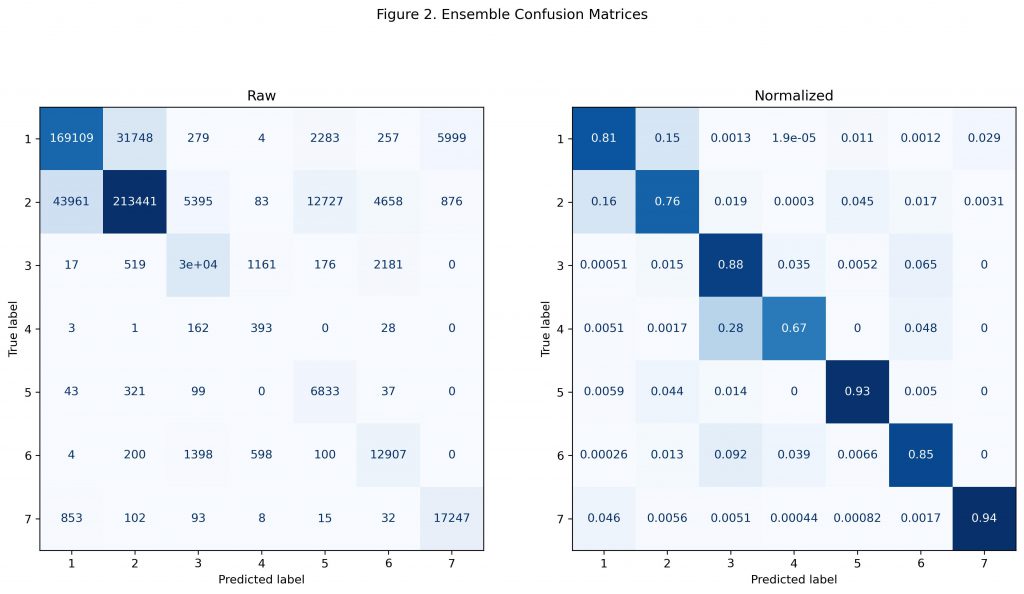
Figure 2 shows the raw and normalized confusion matrices for the final ensemble. As shown in the raw matrix, the greatest number of incorrect predictions come from mistakes between the first two cover types. This is not surprising, as they make up the largest portion of the testing dataset. Still, even the tie breaking model that was trained on only these two cover types showed similar mistakes. This suggests that the much larger testing dataset has examples from these two cover types which are unique and not represented during training. The best way to approach this issue in the future would be to randomly select a training dataset that is a greater portion of the overall data, so that a wider variety of trends could be learned.

Even though bootstrapping was used to increase the prevalence of the first two majority cover types, performance on the five minority cover types was still high as shown in the normalized matrix. Only the fourth cover type (Cottonwood / Willow) had lower accuracy than the first two cover types, but this was also the category which had the lowest number of total observations as shown in Figure 1. It could be that with so few observations potentially remaining in the test set, the sample size was too small for a reliable evaluation of performance. Again, generating training and testing data which is more evenly split and representative of a future application would benefit this process.