
Data

Background
As mentioned, this dataset was aggregated for a Kaggle competition and originally comes from sources across the US Geological Survey and US Forestry Service.
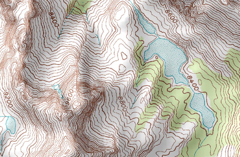
These institutions are charged with both observing the natural environment as well as proactively managing and maintaining it. To aid understanding and potential management in the future, it is of interest to know what factors affect different types of forest growth. This requires that the observed areas be generally free from human interaction so that the natural relationships themselves may be better understood. To this end, isolated sections of the Roosevelt National Forest were divided into 30×30 meter plots to make up the individual data points. The cartographic information of each plot was then determined from existing surveys, resulting in the dataset.
Predicted variable: Forest Cover Type
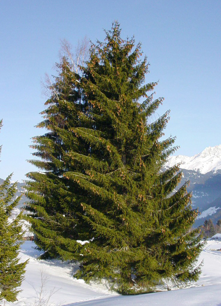
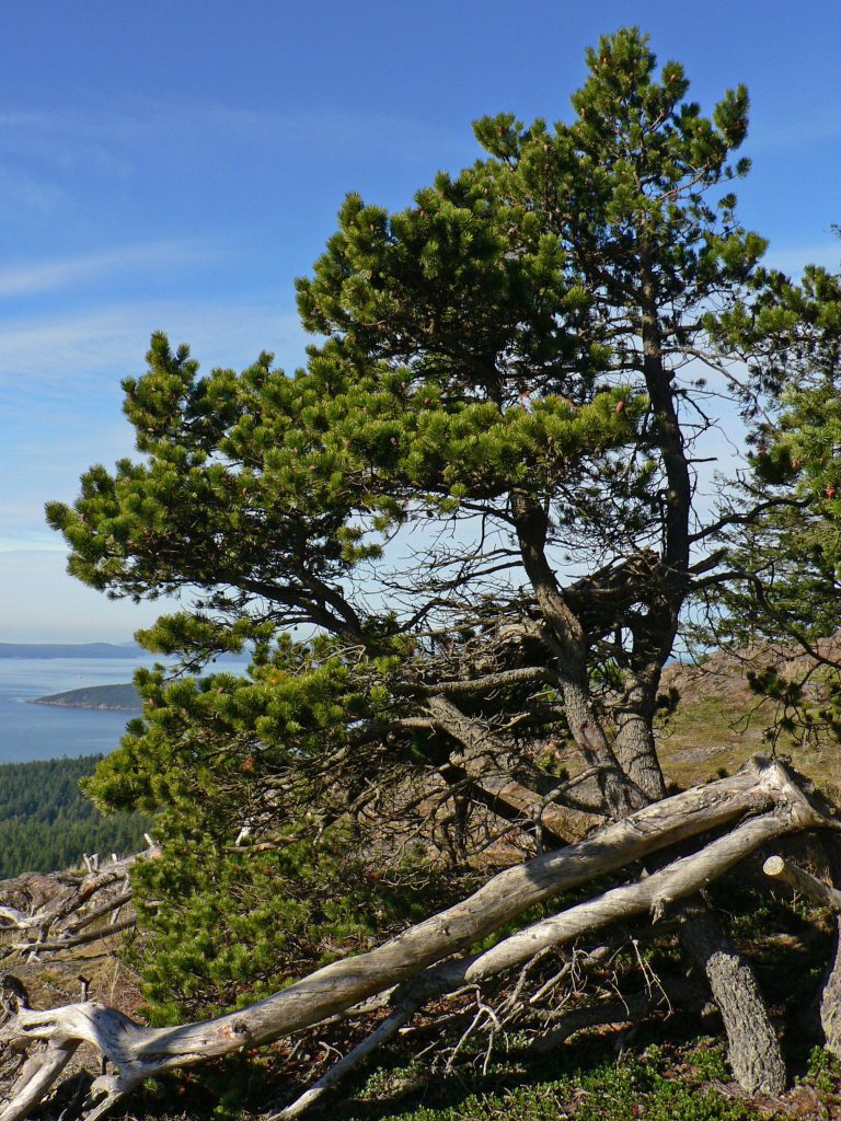
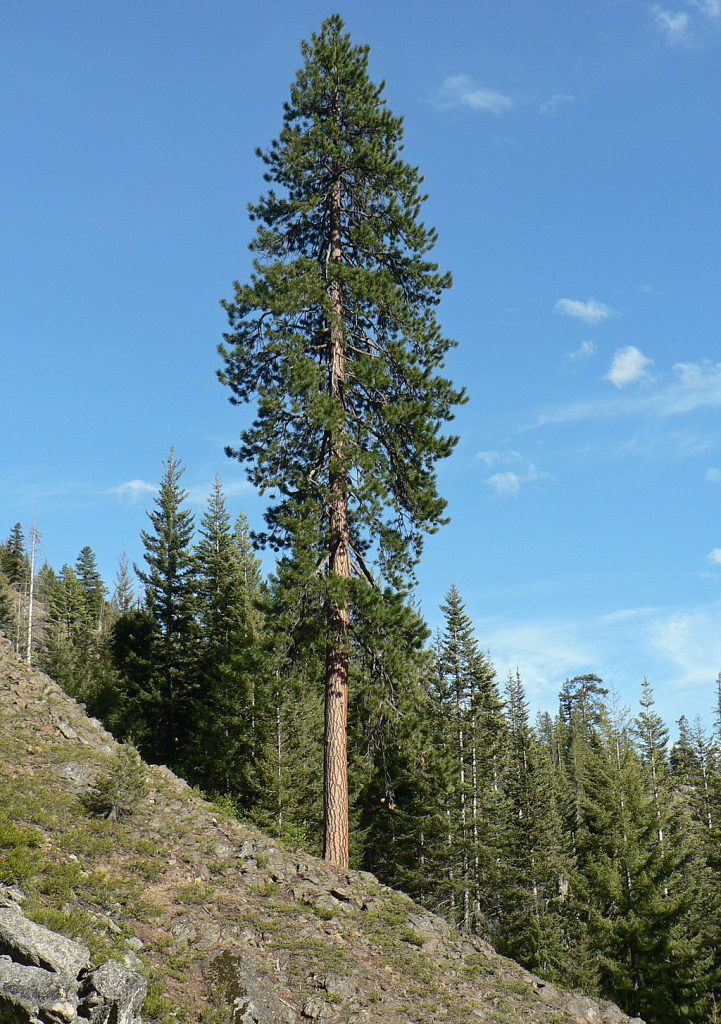
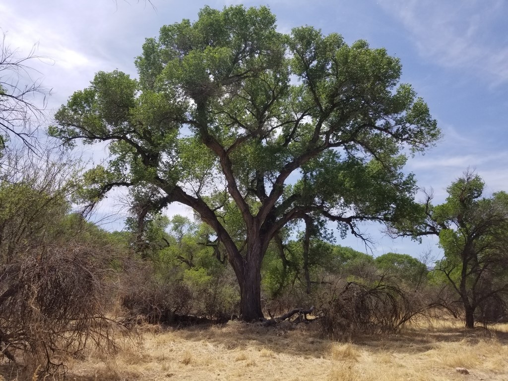
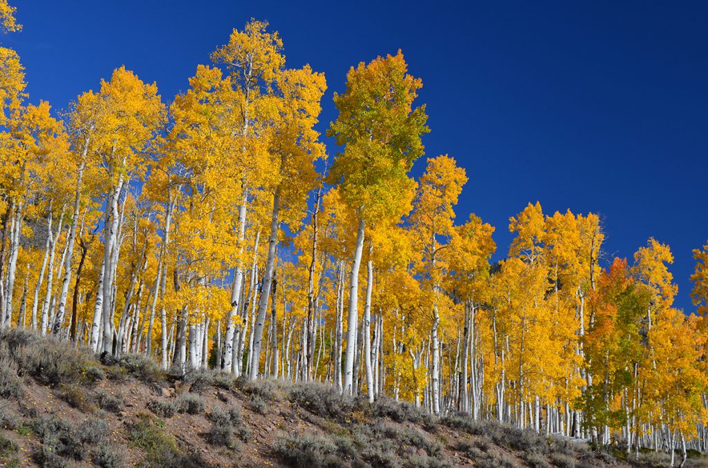
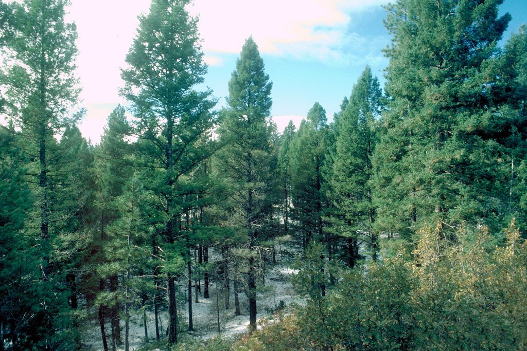
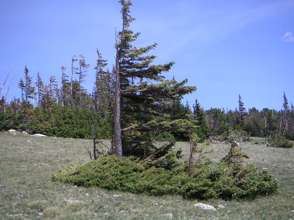
The forest cover type, or predominant type of tree cover, was marked for each 30×30 meter plot. By having insight and predictive power for what tree covers may grow where, better forest management practices may be developed. In total, there were seven different cover types represented within the dataset, shown below.
Predictor variables:
A variety of cartographic variables were available for modeling. For each 30×30 meter plot, the full list of raw variables was:
- Elevation in meters
- Aspect in degrees azimuth
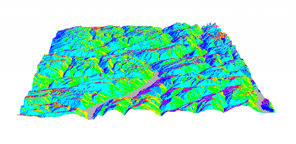
- Slope in degrees above horizontal
- Horizontal distance to nearest water feature, roadway, and fire point
- Vertical distance to nearest water feature
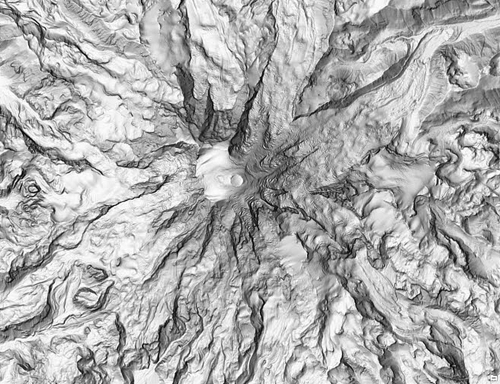
- Hillshade index at 9 AM, 12 PM, and 3 PM
- Wilderness area category
- Soil type category
Given that the dataset was collected within the predefined range of Roosevelt National Forest, wilderness area is an indicator of which out of four major subsections of the Forest the plot came from. Soil type was also a categorical variable, with forty different types which were recorded.
Some of these, such as elevation or soil type, needed little outside information to process. Others, such as the aspect, slope, or Cartesian distances, were much more valuable with certain transformations or in combination. The gallery below shows certain more useful representations that were found when exploring domain knowledge.
Total Distance to Hydrology:
The Cartesian horizontal and vertical distance to hydrology were provided for each plot. In addition to the many ways proximity to water was included, one of the most useful was the total distance. This was found using Pythagorean’s theorem, which calculated the length of the direct line between the plot and the nearest body of water ignoring any intermediate obstacles.
Average Hillshade:
Three different variables provided the hillshade index in the morning, midday, and late afternoon. While these variables were still used individually, taking the average hillshade throughout the day also provided a meaningful input to models. In addition, unlike the name implies a greater hillshade index corresponds to greater surface illumination at vice versa.
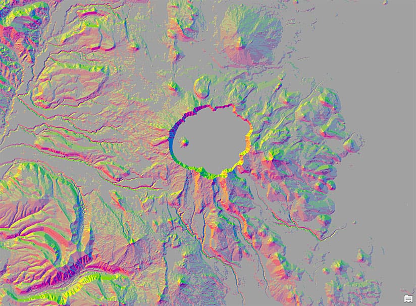
Aspect and Aspect-Slope:
The aspect in degrees azimuth, or degrees clockwise from North, indicated which direction the slope of the plot faced. While normally aspect ranges from 0 to 360 degrees, restricting it to only the 0 to 180 degrees between North and South, regardless of whether the slope faced East or West, also provided value. Given that aspect naturally involves slope, different functions of both variables were also investigated.
Continue to the Models page next to see how the dataset provided opportunities and challenges for this task. Select exploratory data analysis is presented in conjunction with how models performed on the Analysis page.
Dataset Citation:
Bache, K. & Lichman, M. (2013). UCI Machine Learning Repository. Irvine, CA: University of California, School of Information and Computer Science