Still, this estimate must be qualified by the large confidence interval ranging from one to all six primary O-rings failing. In both Figures 4 and 5, the width of the Wald confidence intervals generally increases as temperature decreases in the full model. In the binary model of Figure 4, however, the confidence interval shrinks as temperatures decreases extremely. In fact, at the launch temperature of 36°F the width is extremely small in the binary model. This represents high confidence that at least one O-ring will fail. However, this is likely an example of a “zero-width” interval being estimated due to failing to meet the Wald interval assumptions for a Binomial distribution. The width of the confidence interval ranging to below zero and greater than one is a similar a demonstration of its failure in the current context.
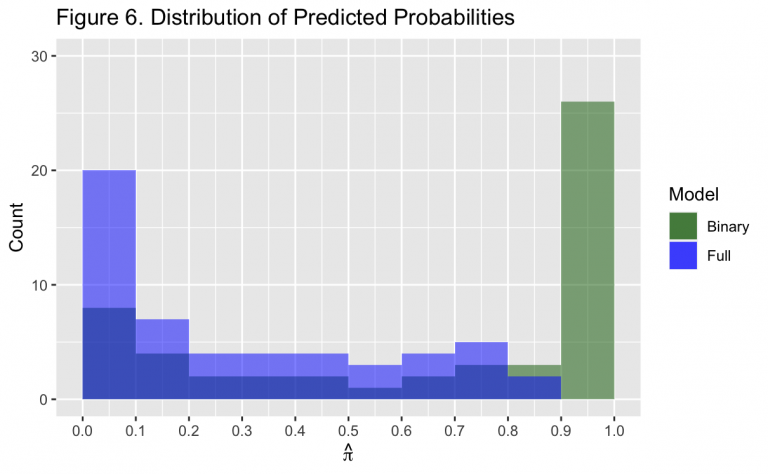
The validity of the Wald intervals can be examined via Figure 6. Specifically, the Wald interval assumes the outcome variable follows a Normal distribution and has a large sample size. Earlier in the exercise, however, a Binomial distribution was assumed for a more appropriate and useful model. While Binomial distributions resemble normal distributions when n is large and p is near 0.5, these circumstances are not usually met and lead to “chaotic coverage” of the Wald interval.^{[3]} Also as noted earlier, Space Shuttle launches are rare events and the overall size of the dataset is small at less than thirty observations.
The effect of these differences can be seen in Figure 6 where \hat{\pi} has fewer observations towards the center of its range, with a greater number on its edges. This is true for both the binary and full models. However, this is the opposite of a Normal distribution where the median value is the most often observed. With all of these differences, the Wald intervals should not be considered precise estimates of the standard error.
As done with the previous hypothesis tests, the profile LR confidence interval can be constructed instead of the Wald. Unlike the Wald, the LR confidence interval assumes a \chi^2 distribution in the outcome. This is much more easily approximated by the Binomial distribution the data was assumed to follow for modeling, as found when comparing a \chi^2 distribution to Figure 6.
At 36°F, the probability of an individual O-ring failing has a 95% LR confidence interval of 12.6% and 97.4%. The Wald confidence interval under the same conditions is 14.3% and 97.4%. While a small difference at this temperature, this demonstrates that the LR interval is more conservative than the Wald and should be preferred.
Dalal et al., the authors of the publication this exercise is based on, did not use Wald or LR methods to estimate error. Instead, they used a parametric bootstrap. Bootstrapping involves randomly varying a quantity of interest for many iterations, where a new outcome is calculated for each iteration. After many iterations, a distribution of possible results is generated. By the central limit theorem, this distribution is approximately Normal. Once constructed, the distribution’s variance can then be used as an estimate of uncertainty in the outcome as a function of the varied quantity.
Because one of the key features of this dataset is the low number of observations, at 23 total, it may be assumed that this is a primary contributor to error in a model’s predictions. From this, a procedure was designed where each iteration would:
- Sample the original dataset with replacement to create a new synthetic dataset of equal size (23 observations)
- Fit a model with identical structure to the new dataset
- Make a prediction using the new model at a temperature of interest
After a large number of iterations, the variance in the predictions would then be used to construct the confidence interval at the given temperature. In this context, an accurate confidence interval for the temperature of the Challenger‘s final launch at 36°F is desired. Because no prior observation was from such a low temperature, this also represents an estimate of the out-of-sample uncertainty. For comparison, the procedure is also repeated at a temperature of 70°F to demonstrate an in-sample estimate.
Similar to before, the probability of an individual O-ring failing at the launch temperature of the Challenger was estimated via parametric bootstrap to be 66.4%. The bootstrapped 95% confidence interval was 16.2% and 116.6%. At 70°F, the same method estimated the probability at 4.6% with a 95% confidence interval of 0% and 9.2%. Note that in both of these intervals, bounds can extend beyond the limit of 0% and 100% similar to the Wald interval. Although bootstrapping has become popular in recent decades with the rise of computation power and simple application to many contexts, certain issues can such as this still be encountered depending on the use case.
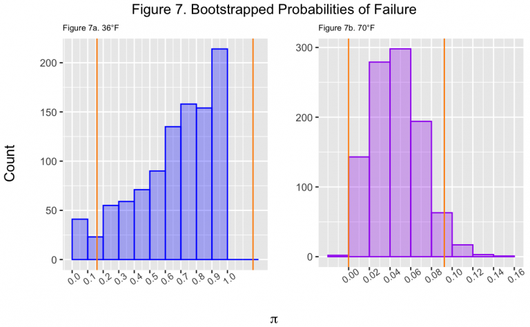
Figure 7 shows the bootstrapped probabilities of failure for a single O-ring at 36°F and 70°F. The confidence intervals determined from the distribution are also shown in orange for each temperature. The “parametric” nature of the bootstrap can be observed as both resemble a Normal distribution, although the boundaries at 0% and 100% add a slight skew. However, these are both much more similar to a Normal distribution than what is shown in Figure 6, suggesting the bootstrap is more reliable than the Wald intervals even though both have similar boundary problems. To fix this in the future, the exact Clopper-Pearson interval for a Binomial distribution should also be investigated.
Linear Regression
While a Binomial distribution was assumed for the outcome and used with a logit link function, a simpler approach may have been to use only standard linear regression with a Gaussian distribution and identity link function.
\hat{\pi}=\hat{\beta_0}+\hat{\beta_1}(Temp)
Shown above, a linear model may follow a very similar form to the Binomial models previously considered. Like the Binomial models, it also finds that temperature is significant for the presence of an O-ring failure with \hat{\beta_1} = -0.079 at a p-value less than 0.05. This also implies there is an inverse relationship between the two variables, where the likelihood of an O-ring failure increases as the temperature decreases. Specifically, with all else constant, decreasing the temperature by 10°F would increase the probability of an individual O-ring failure by ~7.9%.
Even though a similar result is found, this model should not be used instead of the Binomial model. Chiefly, this is because the linear model does not have bounds on the output so that sometimes a probability greater than one or less than zero may be predicted. Although previous confidence intervals were found to have this problem, this was due to the calculation of the standard error and not the model itself. In this linear model, a probability of one is reached at about -48°F while a probability of zero is reached at about 78°F. Given that there were recorded launches above this maximum temperature, and one at 75°F had O-ring failures, this is a very undesirable property of the model.
In addition, the linear model assumes homoscedasticity. This means that the variance in the model’s residuals should be constant both over the range of the dependent variable as well as the domain of the independent variables.
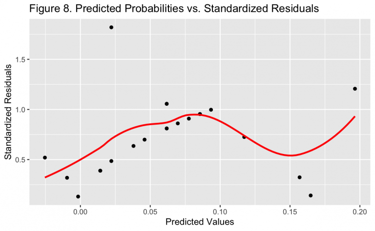
Shown in Figure 8, the standardized residuals are not constant over the range of the dependent variable in the model, failing to meet the homoscedasticity assumption. This result was expected, however, as it can be shown that the variance in a random variable from a Binomial distribution is a function of itself, or Var(\pi) \propto \pi*(1-\pi). It can be further seen in Figure 8 that there is a general upward trend as \pi \to 0.5, which follows from the variance relationship. Given that the homoscedasticity assumption is not met, there is further reason to prefer the Binomial model to the linear regression.