With the given context, there are different possible approaches to estimate the relationship between the environmental variables and O-ring failure. Given that each O-ring is discrete, a Poisson or Binomial distribution could be used depending on the modeling goals. The Poisson distribution describes processes which, among other things, occur over an interval at a constant average rate. This could be used to model the expected count of O-rings which fail for a series of Space Shuttle launches. However, the focus on the average over time is not particularly useful to estimate failure in a specific future launch. The Binomial distribution, on the other hand, describes processes which contain several binary events. This fits well with the success or failure of multiple O-rings within a single Shuttle launch. It also would be more fitting for predicting the probability of failure on a single launch in the future, such as the Challenger at the start of its final mission. Because of this, only the Binomial distribution will be used in this investigation.
For both the Poisson and Binomial distributions, an assumption of independence is required. As part of this, it would be necessary that each Space Shuttle launch is independent and identically distributed (IID) compared to all others. In general this should be true, although there may be minor reasons why this is violated. For example, over time Shuttle technology or launch procedures may have been improved based on prior experience. This would be equivalent to a distributional change over time. In addition, part of the reason SRBs were recovered was not just for observing O-ring damage, but also for refurbishment and potential re-use in later launches. Having sets of launches with the same SRBs could result in correlated observations that bias any resulting estimates. It could also be expected that re-used SRBs in general cause greater O-ring damage than those which are new. This would likewise cause bias because it involves the observed outcome of O-ring failure. With either a Poisson or Binomial distribution, these must all be assumed to be negligent. In the future, knowledge of which SRBs were re-used for which launches could be incorporated into modeling for a more accurate estimate.
These modeling options also require that in addition to each Shuttle launch being IID, each of the six O-rings for any given flight must be IID as well. If the O-rings were not independent, the failure of a given O-ring would not only be a function of the environmental variables but also of the failure of other O-rings. Consequently, there would not be just one relationship between the O-ring failure and the environment, but multiple relationships depending on which O-ring was under consideration. Similarly, if they were not identically distributed, then different O-rings could have their own relationships to the environmental variables rather than a single relationship for all O-rings.
Just like with the IID Shuttle launches, this is avoided with the assumption of independence. However, it may not be completely valid. For example, the six O-rings are spread out across two SRBs for each launch. It might be that there are small differences between specific SRBs with respect to the stress the O-rings experience. In particular, one might have minor manufacturing differences that puts more stress on its O-rings compared to the other. This would result in a non-identical distribution, with the same complicating effects previously mentioned. Therefore, it is likely that every O-ring is not perfectly IID but this must be ignored for the sake of the model.
With the assumption of independence, two different uses of the Binomial distribution will be investigated. The first will model n = 6 IID O-rings for every launch, where each O-ring has an identical probability p of failure. The set of O-rings within each Shuttle launch and the series of all launches will then make up a Bernoulli process. This will be referred to as the “full” outcome throughout this report. The second will investigate only the probability of a launch experiencing any O-ring failures by use of the binary distress variable created during the EDA. This will model the reduced n = 1 Bernoulli trial of whether at least one O-ring failed on a given launch, with a single probability p of this occurring. This is a special case of the Binomial distribution known as the Bernoulli distribution, and will be referred to as the “binary” outcome throughout this report.
An advantage of the former is that it uses all available information in the dataset, potentially estimating a more accurate relationship between O-ring failure and environmental conditions. It also can provide a more useful prediction for the outcome of the Challenger disaster, since any design-flaw in a secondary O-ring when the primary fails would cause a catastrophe. Having an estimate of a specific number of primary O-rings which fail would then be proportional to the probability of the catastrophe. The use of the binary distress outcome, however, only estimates if at least one O-ring will fail without regard to how many. Still, because of its simpler nature it can potentially be more precise when the number of observations is so low. Therefore, the full outcome will be used to provide a primary estimate of the disaster’s probability, with the binary outcome used as a spot-check against its results.
Functional Form
There are two explanatory variables of interest, temperature and pressure. To test whether either of these are significant, a series of three models will be created.
logit(\pi) = \beta_0
The first, shown above, will only include an intercept and serve as the null hypothesis where neither temperature nor pressure have a relationship with O-ring distress. This equivalent to \beta_{T} = \beta_{P} = 0.
As common with Binomial distributions, a logit link function will be used to relate the dependent and independent variables. The logit is defined as logit(\pi) = ln(\frac{\pi}{1 – \pi}) where \pi is the probability of the outcome of interest. In the full model, this is the probability of failure of an individual O-ring. In the binary model, it is the probability of failure of at least one O-ring in a launch.
logit(\pi) = \beta_0 + \beta_{T}*T
The second, shown above, will include temperature as the sole independent variable denoted by T. This is motivated by Morton Thiokol’s pre-launch investigation of O-ring condition deteriorating at lower temperatures using the same dataset. Later, it will be shown how their mistakes in treatment of the data would lead to an underestimate of the probability of catastrophe.
logit(\pi) = \beta_0 + \beta_{T}*T + \beta_{P}*P
Finally, the pressure P will be included along with T in the third model to see if both environmental conditions are also significantly related to O-ring distress.
The same set of three models will be used for both the full and binary outcome variables. Note that for the full models, instead of creating n = 6 unique data points for the O-rings of each launch, the fraction of O-ring failures in a single launch was used as the dependent variable. When paired with the weights of each observation, which is constant at six O-rings for all launches, this produces identical model estimates.
Hypothesis Testing
A likelihood ratio test (LRT) will be used to determine whether a model associated with an alternative hypothesis is a significant improvement over the null hypothesis model. If the first alternative hypothesis is significant, i.e. involving only T, then the second alternative hypothesis including both T and P will be assessed against it.
LRTs compare the likelihood of the alternative hypothesis model against the null hypothesis model. In general, for a binary outcome an LRT is mathematically expressed as:
-2log(\Lambda) = -2log( \frac{L(\hat{\mathbf{\beta}}^{(0)} | y_1, \dots, y_n)}{L(\hat{\mathbf{\beta}}^{(a)} | y_1, \dots, y_n)} = -2\sum y_i log\left( \frac{\hat{\pi}_i^{(0)}}{\hat{\pi}_i^{(a)}} \right) + (1 – y_i ) log\left( \frac{1- \hat{\pi}_i^{(0)}}{1- \hat{\pi}_i^{(a)}} \right)
Where:
– \Lambda is the likelihood ratio test statistic
– L() is the likelihood function of the estimated model given the data, which in this case involves cross entropy between the predicted probabilities and binary true values.
– \hat{\pi}_i^{(0)} is the estimated probability of success of Bernoulli trial i under the null hypothesis H_0
– \hat{\pi}_i^{(a)} is the estimated probability of success of Bernoulli trial i under the alternative hypothesis H_a
Because of these planned, repeated hypothesis tests, the Bonferroni correction will be applied to strengthen the level of significance required to reject the null hypothesis. Starting from \alpha = 0.05, with four comparisons between the alternative and null hypothesis models, the new p-value required for significance will be \alpha = 0.05 / 4 = 0.0125.
When performing the LRTs including only temperature in the alternative hypothesis, p-values of 0.0048 and 0.0132 are found for the binary and full models respectively. The binary model is definitively past the threshold required for significance of 0.0125, but the full model is very slightly above. While this would normally result in a failure to reject the null hypothesis, often times the choice of interpretation is dependent on the testing context and broader considerations. In particular, methods for defining significance should be viewed as guidelines rather than hard and fast rules. In this case, the Bonferroni correction is known for being overly conservative in that it guarantees the family wise Type I error rate will always be less than the desired level of \alpha. In particular, strict adherence to the Bonferroni correction is known for higher Type II error rates, or failure to reject a false null hypothesis. The significance of temperature in the binary model also suggests this could be the case if judging the borderline full model as non-significant. Therefore, for being nearly at the threshold and with these considerations, this result will still be taken as significant.
With the first pair of alternative hypotheses failing to be rejected, they now will take the position of the null hypothesis for comparison against including pressure. For these LRTs, p-values of 0.2156 and 0.2145 are found for the binary and full models respectively. Unlike the previous borderline case, both of these are well above the Bonferroni corrected significance level as well as the original \alpha. Therefore, the null hypothesis that pressure does not have a significant relationship with O-ring failure is failed to be rejected. Moving forward, the temperature-only models will be used for further investigation and prediction.
Model Results
Before making a prediction, the fitted parameters within the model may also be examined. In this case, \beta_T may be interpreted for the relationship between temperature and O-ring failure. When doing so with any link function other than the identity link, changes in an independent variable must account for additional transformation(s) to find the change in the dependent variable.
OR = \frac{Odds_{T + c}}{Odds_T} = \frac{\pi_{T+c}}{1-\pi_{T+c}}*\frac{1-\pi_T}{\pi_T}= \frac{exp(\beta_0 + \beta_T*(T + c))}{exp(\beta_0 + \beta_T*T)} = exp(\beta_T * c)
With a logit link function, changes in an independent variable are most commonly interpreted through the odds ratio (OR), with a derivation for this model shown above. Specifically, the example shown describes the OR as a function of a c °F increase in temperature. Previously, the coefficient of temperature \beta_T was estimated to be about -0.232 in the binary model and -0.116 in the full model. Both are negative, implying that generally as temperature increases then the estimated odds of O-ring failure decreases. Conversely, as temperature decreases then the estimated odds of O-ring failure increases.
For a 10°F decrease in temperature, the OR would be about 10.2 in the binary model and 3.2 in the full model. Put into context, this implies that with a 10°F lower temperature the odds of any O-ring failure increases by 10.2 and the odds of an individual O-ring failure increases by 3.2. This change is irrespective of the starting temperature, and as the change in temperature grows more negative then the odds of O-ring failure will continue to increase.
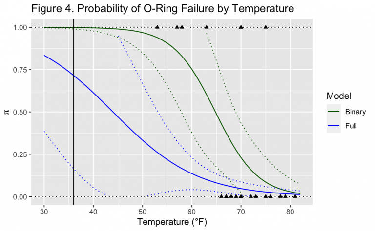
Figure 4 shows the probability of O-ring failure from both models over a range of temperatures. The Wald confidence intervals with \alpha = 0.05 are shown as dotted lines for each model. Previous Shuttle launches are also included depending on whether they did or did not have at least one O-ring failure, which is the dependent variable in the binary model. Finally, the vertical line represents the launch temperature of the Challenger disaster of 36°F.
As described previously the binary case represents the probability that any of the six O-rings will fail during launch, while the full case represents the probability of an individual O-ring within the six failing. Shown earlier with the OR, a decrease in temperature increases the probability of O-ring failure in both models. Throughout the entire range of temperatures, the binary model has a greater probability than the full model. This is intuitive as it only tracks the probability of whether at least one out of the six O-rings per launch will fail, rather than the probability of failure in a specific individual O-ring.
At the launch temperature of the Challenger, the binary model predicts there is a near guarantee that at least one O-ring will fail. The full model likewise predicts a high probability of each individual O-ring failing at nearly 75%. With the O-rings being assumed IID as required for the Binomial distribution, the expected number of O-ring failures on a single launch is then given by:
E[Y] = n * p = 6 * \hat{\pi}(T)
where n = 6 from the six IID O-rings on each launch and p = \hat{\pi}(T) is the estimated probability of an individual O-ring failing at a specific temperature as given by the full model. Again, by design only the full model can estimate how many O-rings on a given launch may fail. The binary model is only useful for understanding if at least one O-ring will fail, without regard to the total number.
Original Mistakes
A key feature of Morton Thiokol’s original analysis was that all launches which had zero O-ring failures were omitted.^{[1]} This was justified by assuming they had nothing to offer to an understanding why O-rings may fail, or if temperature could be related. However, to falsify the claim that temperature is related to O-ring failure, both successes and failures of O-rings must be considered. Attempting to do so only based on examples of O-rings which failed, or conversely O-rings which did not fail, is impossible. Especially when a causal effect is suspected, an analysis which attempts to do so does not meet fundamental criteria of science.
An identical subset of the launch data as used by Morton Thiokol can be replicated. With this, the same structure of the full model can be fit to determine how it may impact analysis.
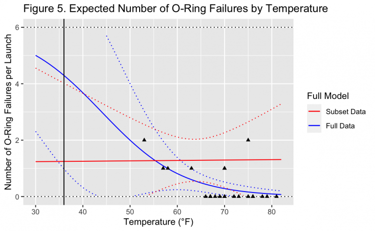
Figure 5 shows the number of predicted O-ring failures per launch over a range of temperatures, along with the Wald confidence intervals. The two curves are both generated from the full model, one which uses only the data subset Morton Thiokol considered and one on the full data. Like Figure 4, the vertical line indicates the launch temperature on the morning of the Challenger disaster of 36 °F.
Most notably, using only the subset data implies that temperature is not related to O-ring failure. Instead, the predicted number of failures is constant around one. At higher and lower temperatures the Wald confidence interval grows wider, but this is due to a lack of observations outside of the six which remain. This also highlights that in addition to being biased, this subset is incredibly small. When already starting with rare events such as Space Shuttle launches, any further reduction in dataset size must be well motivated. As a result, with only six observations and two parameters in the model, the available degrees of freedom are nearly exhausted.
On the other hand, the full model with all data tracks previous Shuttle launches well. The only point which does not fit this curve is the observation with two O-ring failures at a temperature of about ~75°F. Even though this point is far from the predictions of the model, it does not appear to have skewed its fit.
Importantly, the model with all data predicts that about four out of the six primary O-rings would fail at the launch temperature of the Challenger. This is an key result, as no previous launch had greater than two O-ring failures observed. As mentioned earlier, these six primary O-rings were intended to be redundant with six secondary O-rings. However, early in the Shuttle program it was known that a phenomena specific to the secondary O-rings could occur which rendered them useless at the start of each launch. If this happened at the same time as a primary O-ring failed, then it was already known that the result would be a catastrophe. Therefore, with four primary O-rings expected to fail at launch, the Challenger disaster would only have been averted if all four of the secondary O-rings to these did not also start the launch non-functional.